The Falcons Should Have Attempted an Onside Kick to Start Overtime

After losing the overtime coin toss, the Atlanta Falcons were forced to kick off to the New England Patriots to open the first overtime in Super Bowl history. They kicked deep into the end zone, resulting in a touchback and Patriots ball at the 25-yard line. Tom Brady and co moved the ball straight downfield with little resistance and scored a touchdown, ending the game and capping off the largest comeback in Super Bowl history. Kicking deep gave the ball right back to the quarterback many consider the GOAT and sealed the Falcon's fate.

But what if Atlanta had attempted an onside kick?

Per the NFL's current overtime rules, if the kicking team successfully recovers an onside kick the game immediately becomes sudden death:

A.R. 16.2 ONSIDE KICKOn the opening kickoff of overtime, Team A legally recovers the ball at the A41.Ruling: A's ball, first-and-10 on A41. A kickoff is considered an opportunity to possess for the receiving team. Team B is considered to have had an opportunity to possess the ball.

Their decision to kick off resulted in NE with the ball at their own 25, which will serve as our "control scenario", where ATL had a 35.6% chance to win (per Prediction Machine):

Whether "Momentum" Exists in College Football

One of the biggest questions in sports has long been whether momentum in sports actually exists. It's an argument that splits along the classic "statisticians vs traditionalists" lines; the numbers imply that momentum isn't real, while athletes subscribe to the notion that it exists, as do sportscasters, talking heads, etc. It makes sense to believe in it: you want every possible advantage as a competitor, and if you're promoting an event you want to illustrate the most compelling story possible.

But what if it's just randomness?

I gathered the data on every college football game from this past season, resulting in 872 games (including FCS opponents). I filtered down to only FBS vs FBS, resulting in 774 games.

There were 6,975 scores (defined as a TD, FG, or defensive score, so that extra points don't count twice) in this past season. I removed the 774 that were the first score of the game, leaving me with 6,201 to analyze. I split these between "momentum scores", i.e. scores that followed a score by the same team, and "counter scores", i.e. scores that followed a score by the other team. The initial results seemed pretty damning:

Total Scores	6,201
Momentum Scores	2,802	45.19%
Counter Scores	3,399	54.81%

Not only does momentum not appear to exist, but this seems to show evidence against it! That being said, the opposing offense almost always gets the ball next (barring an onside kick or a turnover on the kick return). This obviously greatly increases the chance of a "counter score" since the other offense has the ball, unless we believe that "momentum" affects both the offense and defense on the same team. The above data seems to strongly counter that hypothesis; testing this against the assumption that "momentum" or "counter" scores occur at a 50/50 rate results in a z-score of -7.62, which translates to a 0.0000000000013% chance that that hypothesis is correct.

So how can we prove whether momentum exists or not? That's a tall task, so my focus is more on showing whether there is an actual trend that occurs, or whether it's likely randomness. 

To illustrate this, think about a series of 100 coin flips. You would expect there to be 50 heads and 50 tails (this is the "expected value") at the end, but this isn't always the case due to natural variance (i.e. randomness). Even within this series you will see streaks due to this randomness: if you flip a coin 3 consecutive times, the odds of seeing 3 heads in a row is 1/8, or 12.5%. But overall, there is almost a 99% chance that you will see 3 consecutive heads in those 100 flips.

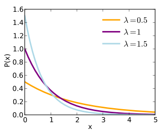
I took this idea and applied it to streaks of scores, meaning the number of consecutive times one team scored without their opponent scoring. I hypothesized that these streaks would follow the exponential distribution, which has the following density function and graph:




Setting λ = 0.9 results in the following comparison between what actually occurred in the data, Actual f(x), and what the theoretical function returns, Expected f(x):

Streak	Frequency	Actual	Expected
1	3399	0.548	0.603
2	1556	0.251	0.245
3	659	0.106	0.100
4	294	0.047	0.041
5	142	0.023	0.016
6	72	0.012	0.007
7	44	0.007	0.003
8	22	0.004	0.001
9	11	0.002	0.000
10	2	0.000	0.000

Graphing these functions together show that they are almost completely superimposed on one another:

The only "streak" that differs significantly from the theoretical function is a streak of 1, which might be explained by the previously described fact that the opposing team usually gets the ball following their opponent's score. It certainly seems that the exponential distribution fits this data, thus indicating that momentum does not actually exist (in college football), but is rather a construct of trying to explain randomness.

UNC's Top 3 Scorers in Close Games vs Blow Outs

Carolina's top 3 most important offensive players are Justin Jackson, Joel Berry III, and Kennedy Meeks, as supported by KenPom's offensive rating, which measures "the number of points produced by a player per hundred total individual possessions" (originally created by Dean Oliver):

Player	ORtg
J Jackson	125
J Berry III	123
K Meeks	116

One perceived characteristic of these scorers is they seem to pad their stats in blowouts, but don't come through as often in close games. There has been some work done on quantifying "clutch", but this isn't what I'm trying to do here. I just want to determine if these three truly do shoot better or worse depending upon how close the game is.

Of course, this evokes a "chicken or the egg" problem: do we shoot more poorly in games that are close, or does our poor shooting lead to closer games? I first looked at two metrics split between wins and losses: offensive rating (as mentioned previously) and eFG, which gives more weight to 3-pointers:

	ORtg			eFG
Player	W	L	Diff	W	L	Diff
J Jackson	126	119	7	54.90%	57.84%	-2.94%
J Berry III	132	76	56	59.41%	31.92%	27.48%
K Meeks	119	111	7	52.79%	48.41%	4.38%

The biggest conclusion that jumps off the page here is something I wasn't even looking for: how important Berry is to whether we win or lose. He has been markedly worse in every loss except for Kentucky (which was 50/50 down to the end and could have gone either way). As Berry goes offensively, so does the win/loss column (we also struggled mightily in two games he missed, narrowly beating Davidson and Tennessee at home).

We only have 4 losses though, so how do things look on a more macro view over all of our games, based on the margin of victory (or defeat)? I bucked the average offensive ratings for each player based on the margin of victory:

This illustrates two things:

1. As shown before, Berry is significantly worse in our losses (bucket [-15 to -1])
2. Jackson's efficiency drops by a lot in close wins (bucket [0, 5])

Meeks is remarkably consistent across all games, and Berry is still above average (which is 104.1 this season) in all wins, even though there's some variability in his performance. This isolates Jackson, who has a large drop off in performance in close wins (a margin of victory between 0 and 5). 

This could be variance in the short run, but this picture suggests that Berry and Jackson's poor offensive performances are correlated with losses and close wins, respectively.